Digital Image Processing part3

Dam Construction

• Dam construction is based on binary images. The simplest way to construct dams separating sets of binary points is to use morphological dilation.

Basics to construct dam using dilation

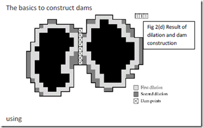
The basics to construct dams using dilation are illustrated in Fig 2.

• Fig 2(a) shows the portions of two catchment basins at flooding step n-1

and Fig 2(b) shows the result at the flooding step, n.

• Dam should be constructed to avoid the spilling of water from one basin to the other.

• Let M1 and M2 denote the sets of coordinates of points in two regional minima. Cn-1(M1) and Cn-1(M2) denote the set of coordinates of points in the catchment basin associated with these two minima at stage n-1 of flooding. These are the two black regions shown in Fig 2(a).

• C[n-1] be the union of these two sets. There are two connected components in Fig 2(a) and one connected component in Fig 2(b).

• Here two connected component encompasses to become single component indicates that water between the two catchment basins has merged at flooding step n. This is denoted by q.

• The two components from step n-1 can be extracted from q by performing the simple AND operation q C[n-1]. All points belonging to an individual catchment basin form a single connected component.

• The connected components is dilated as shown in Fig 2(c) a structuring element by two conditions,

1. The dilation has to be constrained to q (the center of the structuring element can be located only on points in q during dilation) .

2. The dilation cannot be performed on points that would cause the sets being dilated to merge (single component).

• Fig 2(d) shows that a first dilation pass (light gray) expanded the boundary of each original connected component. Condition 1 was satisfied by every point during dilation, and condition 2 did not apply to any point during the dilation process; thus the boundary of each region was expanded uniformly.

• In second dilation (medium gray), several points failed condition 1 while meeting condition 2, resulting in the broken perimeter shown in Figure. Points in q that satisfy the two conditions describes the one-pixel-thick connected path shown crossed-hatched in Fig 2(d) which constitutes the desired separating dam at stage n of flooding.

• Construction of dam at this level of flooding is completed by setting all the points in the path just determined to a value greater than the maximum gray-level value of an image.

• The height of all dams is generally set at 1 plus the maximum allowed value in the image.

• This will prevent water from crossing over the part of the completed dam as the level of flooding is increased.

• Dams build by this procedure are connected components (eliminates the problem of broken segmentation lines).

Watershed Segmentation Algorithm

1. Let …….. be sets denoting the coordinates of the points in the regional minima of an image g(x,y).

2. Let be a set denoting the coordinates of the points in the catchment basins associated with regional minimum [min and max is used to denote minimum and maximum]. represents the set of coordinates for which i.e..

lying below the plane  .

3. The topography will be flooded in integer flood increments, from =min+1 to =max+1.In flooding process, the algorithm needs to know the number of points below the flood depth. Suppose the coordinates in that are below the plane are marked black, and all other coordinates are marked white.

4. Let denote the set of coordinates of points in the catchment basin associated with minimum  that are flooded at stage . Binary image of

Elements in both and are never replaced during execution of algorithm and that two elements in these two sets either increases or remains the same as increases.

• is a subset

• is subset of

• is subset of

• Further flooding would cause the water level in these catchment basins to merge. Thus a dam must be built within q to prevent overflow between the catchment basins.

• Algorithm efficiency is improved by using only values of n that correspond to existing gray-level values in ; we can determine these values, as well as the values of min and max, from the histogram of .

The Use of Markers

• Problem with basic watershed algorithm is over segmentation due to noise and other local irregularities of the gradient.

• This results in making a large number of segmented regions useless.

• Solution to this problem is to limit the number of allowable regions by incorporating a preprocessing stage designed to bring additional knowledge into the segmentation procedure.

• Over segmentation can be control by a concept called markers. A marker is a connected component belonging to an image.

• Internal marker is used for objects and external marker for background.

• Two principal steps of marker selection

1. Preprocessing

2. Definition of a set of criteria that markers must satisfy.

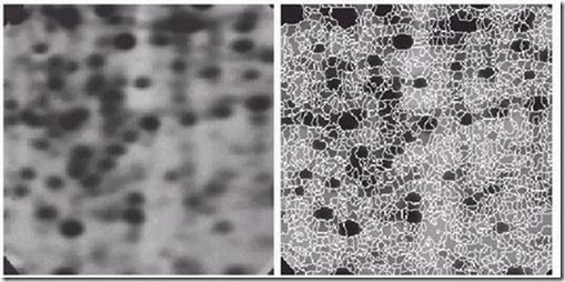
Fig 4 (a) Electrophoresis image, (b) Result of applying watershed segmentation algorithm to the gradient image (over segmentation).

Fig 5 (a) internal marker image (light gray regions) and external markers (watershed lines)

(b) Result of segmentation.

• We define an internal marker (1) a region that is surrounded by points of higher altitude (2) such that the points in the region form a connected component and (3) in which all the points in the connected component have the same gray-level value.

• After the image was smoothed, the internal markers resulting from this definition are shown as light gray, blob like region in Fig 5(a).

• Next watershed algorithm was applied to the smoothed image, the restriction that these internal markers be the only allowed regional minima.

• Fig 5(a) shows the resulting watershed lines defined as the external markers. The external markers partition the image into regions, with each region containing a single internal marker and part of the background.

• Now apply watershed segmentation algorithm to each individual region; Fig 5 (b).

• The point is that using markers brings a priori knowledge to bear on the segmentation problem.

• The fact that segmentation by watersheds offers a framework that can make effective use of this type of knowledge is a significant advantage of this method.

Matching

• Matching is another basic approach to segmentation that can be used to locate known objects in an image, to search for specific patterns, etc.

• The best match is based on some criterion of optimality which depends on object properties and object relations.

Fig 1: Segmentation by matching; matched pattern and location of the best match.

• Matched patterns can be very small, or they can represent whole objects of interest.

• While matching is often based on directly comparing gray-level properties of image sub regions, it can be equally well performed using image-derived features or higher-level image descriptors.

• In such cases, the matching may become invariant to image transforms.

• Criteria of optimality can compute anything from simple correlations up to complex approaches of graph matching.

Matching criteria

• Exact copy of the pattern of interest cannot be expected in the processed image - some part of the pattern is usually corrupted in real images by noise, geometric distortion, occlusion, etc.

• Search for locations of maximum match is appropriate.

Match based segmentation Algorithm

1. Evaluate a match criterion for each location and rotation of the pattern in the image.

2. Local maxima of this criterion exceeding a present threshold represent pattern locations in the image.

• Matching criteria can be defined in many ways; in particular, correlation between a pattern and the searched image data is a general matching criterion.

• Let f be an image to process, h be a pattern to search for, and V be the set of all image pixels in h.

• Possible matching optimality criteria describing a match between f and h located at a position (u,v):

• The "1" added to each denominator to prevents dividing by zero for a perfect match.

• The cost is evaluated at each (u,v) pixel location in the image being processed.

• Possible implementation decisions include whether the pattern is only computed entirely within the image or partial pattern positions when the pattern crosses image borders.

• A simple example of the optimality criterion values is given:

Fig 2: Optimality matching criterion evaluation (a)Image data (b)Matched pattern (c)Values of the optimality criterion

• If a fast, effective Fourier transform algorithm is available, the convolution theorem can be used to evaluate matching.

• The correlation between a pattern h and image f can be determined by first taking the product of the Fourier transform F of the image f and the complex conjugate of the Fourier transform of the pattern h and then applying the inverse transform.

• To compute the product of Fourier transforms, F and must be of the same size; if a pattern size is smaller, zero-valued lines and columns can be added to inflate it to the appropriate size.

• Sometimes, it may be better to add non-zero numbers, for example, the average gray level of processed images can serve the purpose well.

Control strategies of matching

• Match-based segmentation localizes all image positions at which close copies of the searched pattern are located.

• These copies must match the pattern in size and rotation, and the geometric distortion must be small.

• To adapt match-based methods to detect patterns that are rotated, enlarged, and/or reduced, it would be necessary to consider patterns of all possible sizes and rotations.

• Another option is to use just one pattern and match an image with all possible geometric transforms of this pattern, and this may work well if some information about the probable geometric distortion is available.

• Note that there is no difference in principle between these approaches.

• Matching can be used even if an infinite number of transformations are allowed. Let us suppose a pattern consists of parts, these parts being connected by rubber links.

• Even if a complete match of the whole pattern within an image may be impossible, good matches can often be found between pattern parts and image parts.

• Good matching locations may not be found in the correct relative positions, and to achieve a better match, the rubber connections between pattern parts must be either pushed or pulled.

• The final goal can be described as the search for good partial matches of pattern parts in locations that cause minimum force in rubber link connections between these parts.

• A good strategy is to look for the best partial matches first, followed by a

heuristic graph construction of the best combination of these partial matches in which graph nodes represent pattern parts.

• Match-based segmentation is time consuming even in the simplest cases with no geometric transformations, but the process can be made faster if a good operation sequence is found.

• The sequence of match tests must be data driven.

o Fast testing of image locations with a high probability of match may be the first step, then it is not necessary to test all possible pattern locations.

o Another speed improvement can be realized if a mismatch can be

detected before all the corresponding pixels have been tested.

o The correlation changes slowly around the best matching location ... matching can be tested at lower resolution first, looking for an exact match in the neighborhood of good low-resolution matches only.

• The mismatch must be detected as soon as possible since mismatches are found much more often than matches.

• Considering the matching formulae given above, testing in a specified position must stop when the value in the denominator (measure of mismatch) exceeds some preset threshold.

• This implies that it is better to begin the correlation test in pixels with a high probability of mismatch in order to get a steep growth in the mismatch criterion.

• This criterion growth will be faster than that produced by an arbitrary pixel order computation.