Digital Image Processing part2
Algorithm: Inner Boundary tracing
1. Search the image from top left until a pixel of a new region is found; this pixel then has the minimum column value of all pixels of that region having the minimum row value. Pixel
is a starting pixel of the region border. Define a variable
which stores the direction of the previous move along the border from the previous border element to the current border element. Assign
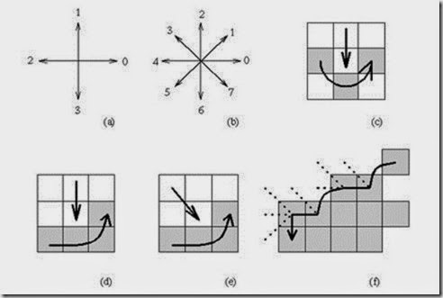
(a) if the border is detected in 4-connectivity (Fig 6(a) )
(b)
if the border is detected in 8-connectivity (Fig 6(b) )
2. Search the 3x3 neighborhood of the current pixel in an anti-clockwise direction, beginning the neighborhood search in the pixel positioned in the direction
The first pixel found with the same value as the current pixel is a new boundary element . Update the value.
3. If the current boundary element is equal to the second border element
, and if the previous border element
is equal to
, stop. Otherwise repeat step 2.
4. The detected inner border is represented by pixels .
Fig 6:Inner boundary tracing (a)Direction notation,4-connectivity (b)8-connectivity (c)Pixel neighborhood search sequence in 4-connectivity (e)Search sequence in 8-connectivity (f)Boundary tracing in 8-connectivity
The above Algorithm works for all regions larger than one pixel.
• Looking for the border of a single-pixel region is a trivial problem.
• This algorithm is able to find region borders but does not find borders of region holes.
• To search for whole borders as well, the border must be traced starting in each region or whole border element if this element has never been a member of any border previously traced.
• Note that if objects are of unit width, more conditions must be added.
• If the goal is to detect an outer region border, the given algorithm may still be used based on 4-connectivity.
• Note that some border elements may be repeated in the outer border up to three times.
Fig 6: Outer boundary tracing
Algorithm: Outer boundary Tracing
1. Trace the inner region boundary in 4-connectivity until done.
2. The outer boundary consists of all non-region pixels that were tested during the search process; if some pixels were tested more than once, they are listed more than once in the boundary list.
• The inner border is always part of a region but the outer border never is.
• Therefore, if two regions are adjacent, they never have a common border, which causes difficulties in higher processing levels with region description, region merging, etc.
• The inter-pixel boundary extracted, for instance, from crack edges is common to adjacent borders; nevertheless, its position cannot be specified in pixel co-ordinates.
• Boundary properties better than those of outer borders may be found in extended borders.
o single common border between adjacent regions
o may be specified using standard pixel co-ordinates
o the boundary shape is exactly equal to the inter-pixel shape but is shifted one half-pixel down and one half-pixel right
Fig 7: Boundary locations (a) Inner (b) Outer (c) Extended.
• The extended boundary is defined using 8-neighborhoods
• e.g.(P) denotes the pixel immediately to the left of pixel P
• Four kinds of inner boundary pixels of a region R are defined; if Q denotes pixels outside the region R, then
• Let LEFT(R), RIGHT(R), UPPER(R), LOWER(R) represents the corresponding subsets of R.
• The extended boundary EB is defined as a set of points P, , , satisfying the following conditions:
• The extended boundary can easily be constructed from the outer boundary.
• Using an intuitive definition of RIGHT, LEFT, UPPER, and LOWER outer boundary points, the extended boundary may be obtained by shifting all the UPPER outer boundary points one pixel down and right, shifting all the LEFT outer boundary points one pixel to the right, and shifting all the RIGHT outer boundary points one pixel down. The LOWER outer boundary point positions remain unchanged.
Fig 9: Constructing the extended boundary from outer boundary (a)Outer boundary (b)Extended boundary construction (c)Extended boundary has the same shape and size as the natural object boundary
• A more sophisticated approach is based on detecting common boundary segments between adjacent regions and vertex points in boundary segment connections.
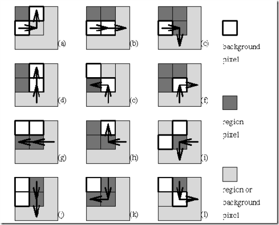
• The detection process is based on a look-up table, which defines all 12 possible
situations of the local configuration of 2 x 2 pixel windows, depending on the previous
detected direction of boundary, and on the status of window pixels which can be inside or outside a region.
Algorithm: Extended boundary tracing
1. Define a starting pixel of an extended boundary in a standard way (the first region pixel found in a left-to-right and top-to-bottom line-by-line image search).
2. The first move along the traced boundary from the starting pixel is in direction dir=6 (down), corresponding to the situation (i) in Fig 10
3. Trace the extended boundary using the look-up table in Fig 10 until a closed extended border results.
• Note that there is no hole-border tracing included in the algorithm.
• The holes are considered separate regions and therefore the borders between the region and its hole are traced as a border of the hole.
Fig 10: look up table defining all 12 possible situations that can appear during extended border tracing.
• The look-up table approach makes the tracing more efficient than conventional methods and makes parallel implementation possible.
• In addition to extended boundary tracing, it provides a description of each boundary segment in chain code form together with information about vertices.
• This method is very suitable for representing borders in higher level segmentation approaches including methods that integrate edge-based and region-based segmentation results.
• Moreover, in the conventional approaches, each border between two regions must be traced twice. The algorithm can trace each boundary segment only once storing the information about what has already been done in double-linked lists.
• A more difficult situation is encountered if the borders are traced in grey level images where regions have not yet been defined.
• The border is represented by a simple path of high-gradient pixels in the image.
• Border tracing should be started in a pixel with a high probability of being a border element, and then border construction is based on the idea of adding the next elements which are in the most probable direction.
• To find the following border elements, edge gradient magnitudes and directions are usually computed in pixels of probable border continuation.
Border detection as graph searching
• Whenever additional knowledge is available for boundary detection, it should be used - e.g., known approximate starting point and ending point of the border
• Even some relatively weak additional requirements such as smoothness, low curvature, etc. may be included as prior knowledge.
• A graph is a general structure consisting of a set of nodes and arcs between the nodes [
, ]. We consider oriented and numerically weighted arcs, these weights being called costs.
• The border detection process is transformed into a search for the optimal path in the weighted graph.
• Assume that both edge magnitude and edge direction information is available in an
edge image.
• Figure 11 (a) shows an image of edge directions, with only significant edges according to their magnitudes listed.
• Figure 11 (b) shows an oriented graph constructed in accordance with the presented principles.
To use graph search for region border detection, a method of oriented weighted-graph expansion must first be defined.
Graph Search Example
• A cost function f( ) must also be defined that is a cost estimate of the path between nodes and (pixels and ) which goes through an intermediate node (pixel ).
• The cost function f( ) typically consists of two components; an estimate of the path
cost between the starting border element and
, and an estimate of the path cost between and the end border element .
• The cost of the path from the starting point to the node is usually a sum of costs associated with the arcs or nodes that are in the path.
• The cost function must be separable and monotonic with respect to the path length, and therefore the local costs associated with arcs are required to be non-negative.
Algorithm: Heuristic Graph search
1. Expand the starting node and put all its successors into an OPEN list with pointers back to the starting node
. Evaluate the cost function f for each expanded node.
2. If the OPEN list is empty, fail. Determine the node from the OPEN list with the lowest associated cost f( ) and remove it. If = then trace back through the pointers to find the optimum path and stop.
3. If the option to stop was not taken in step 2, expand the specified node , and put its successors on the OPEN list with pointers back to . Compute their costs f. Go to step 2.
• If no additional requirements are set on the graph construction and search, this process can easily result in an infinite loop.
• To prevent this behavior, no node expansion is allowed that puts a node on the OPEN list if this node has already been visited, and put on the OPEN list in the past.
• A simple solution to the loop problem is not to allow searching in a backward direction.
• It may be possible to straighten the processed image (and the corresponding graph).
Fig 13: Geometric warping produces a straightened image: The graph constructed requires searches in one direction only (e.g., Top Down).
• The estimate of the cost of the path from the current node to the end node has a substantial influence on the search behavior.
• If this estimate of the true cost is not considered, so no heuristic is included in the algorithm and a breadth-first search is done.
• The detected path will always be optimal according to the criterion used, the minimum cost path will always be found.
• Applying heuristics, the detected cost does not always have to be optimal but the search can often be much faster.
• The minimum cost path result can be guaranteed if
and if the true cost of any part of the path
is larger than the estimated cost of this part
.
• The closer the estimate is to
the lower the number of nodes expanded in
the search.
• The problem is that the exact cost of the path from the node to the end node is not known beforehand.
• In some applications, it may be more important to get a quick rather than an optimal solution. Choosing , optimality is not guaranteed but the number of expanded nodes will typically be smaller because the search can be stopped before the optimum is found.
• If , the algorithm produces a minimum-cost search.
• If , the search will produce the minimum-cost path if and only if the conditions presented earlier are satisfied.
• If
, the search will always produce the minimum-cost path with a minimum number of expanded nodes.
• If
the algorithm may run faster, but the minimum-cost result is not guaranteed.
• The better the estimate of , the smaller the number of nodes that must be expanded.
• A crucial question is how to choose the evaluation cost functions for graph-search border detection.
• Some generally applicable cost functions are
• Strength of edges forming a border
• where the maximum edge strength is obtained from all pixels in the image.
• where DIF is some suitable function evaluating the difference in edge directions in two consecutive border elements.
• Proximity to an approximate border location
• Estimates of the distance to the goal (end-point)
• Since the range of border detection applications is quite wide, the cost functions described may need some modification to be relevant to a particular task.
Fig 14: Graph search applied to coronary vessel border detection. (a) Edge image (b) Determined vessel borders.
• Graph searching techniques offer a convenient way to ensure global optimality of the detected contour.
• The detection of closed structure contours would involve geometrically transforming
the image using a polar to rectangular co-ordinate transformation in order to
`straighten' the contour.
• Searching for all the borders in the image without knowledge of the start and end-points is more complex.
• Edge chains may be constructed by applying a bidirectional heuristic search in which half of each 8-neighborhood expanded node is considered as lying in front of the edge, the second half as lying behind the edge.
Border detection as dynamic programming
• Dynamic programming is an optimization method based on the principle of optimality.
• It searches for optima of functions in which not all variables are simultaneously interrelated.

o Whatever the path to the node E was, there exists an optimal path between E and the end-point.
o In other words, if the optimal path start-point -- end-point goes through E then both its parts start-point -- E and E -- end-point is also optimal.
Fig 18: Dynamic programming: (a) One step of the cost calculation; (b) Graph layers, node notation.
• If the graph has more layers, the process is repeated until one of the end-points is reached.
• The complete graph must be constructed to apply dynamic programming, and this may follow general rules given in the previous section.
• The objective function must be separable and monotonic (as for the A-algorithm); evaluation functions presented in the previous section may also be appropriate for dynamic programming.
Algorithm: Boundary tracing as dynamic programming
Heuristic Graph Search vs. Dynamic Programming
• It has been shown that heuristic search may be more efficient than dynamic programming for finding a path between two nodes in a graph if a good heuristic is available.
• A-algorithm based graph search does not require explicit definition of the graph.
• Dynamic programming presents an efficient way of simultaneously searching for optimal paths from multiple starting and ending points.
• If these points are not known, dynamic programming is probably a better choice, especially if computation of the partial costs is simple.
• Nevertheless, which approach is more efficient for a particular problem depends on evaluation functions and on the quality of heuristics for an A-algorithm. A
• Live wire combines automated border detection with manual definition of the boundary start-point and interactive positioning of the end-point.
• In dynamic programming, the graph that is searched is always completely constructed at the beginning of the search process. Therefore, interactive positioning of the end-point invokes no time-consuming recreation of the graph as would be the case in heuristic graph searching.
• Thus, after construction of the complete graph and associated node costs, optimal borders connecting the fixed start-point and the interactively changing end-point can be determined in real time.
• In the case of large or more complicated regions, the complete region border is usually constructed from several border segments.
• In the live lane approach, an operator defines a region of interest by approximately tracing the border by moving a square window.
• The size of the window is either preselected or is adaptively defined from the speed and acceleration of the manual tracing. When the border is of high quality, the manual tracing is fast and the live lane method is essentially identical to the live wire method applied to a sequence of rectangular windows. If the border is less obvious, manual tracing is usually slower and the window size adaptively decreases.
• If the window size reduces to a single pixel, the method degenerates to manual tracing.
• A flexible method results that combines the speed of automated border detection with the robustness of manual border detection whenever needed.
• Since the graph is only constructed using the image portion comparable in size to the size of the moving window, the computational demands of the live lane method are much lower than that of the live wire method.
• Several additional features of the two live methods are worth mentioning.
o Design of border detection cost functions often requires substantial experience and experimentation.
o To facilitate the method's usage by non-experts, an automated approach has been developed that determines optimal border features from examples of the correct borders.
o The resultant optimal cost function is specifically designed for a particular application and can be conveniently obtained by simply presenting a small number of example border segments during the method's training stage.
Hough transforms
• If an image consists of objects with known shape and size, segmentation can be viewed as a problem of finding this object within an image.
• One powerful global method for detecting edges is called the Hough transform.
• Consider an example of circle detection.
• Search the dark image pixels by this potential center points of the circle can be determined which forms a circle with radius r [Fig 20(b)].
• After the construction of potential circle for all dark pixels of an image the frequency is determined. The true center of the circle is represented by the pixel with the highest frequency [Fig 20:(c)].
• Fig 20(d) presents that the Hough transform can apply to the images with incomplete information or additional structures and noise.
Fig 20: Hough transform(circle detection) (a)Original image (b)Original image of dark circle(radius r) (c)The highest frequency pixel represents the centre of the circle (d)Hough transform detects the circle 9in incomplete and overlapping structures
• The original Hough transform was designed to detect straight lines and curves
• A big advantage of this approach is robustness of segmentation results; that is, segmentation is not too sensitive to imperfect data or noise.
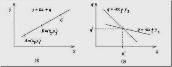
Fig 21: Hough transform principles (a) Image space (b) k, q parameter space.
Fig 22:Hough transform-Line detection (a)Original image (b)Edge image (c) Parameter space (d) Detected lines
This means that any straight line in the image is represented by a single point in the k,q parameter space and any part of this straight line is transformed into the same point.
• The main idea of line detection is to determine all the possible line pixels in the image, to transform all lines that can go through these pixels into corresponding points in the parameter space, and to detect the points (a,b) in the parameter space that frequently resulted from the Hough transform of lines y=ax+b in the image.
• Detection of all possible line pixels in the image may be achieved by applying an edge detector to the image
• Then, all pixels with edge magnitude exceeding some threshold can be considered possible line pixels.
• In the most general case, nothing is known about lines in the image, and therefore lines of any direction may go through any of the edge pixels. In reality, the number of these lines is infinite, however, for practical purposes, only a limited number of line directions may be considered.
• The possible directions of lines define a discretization of the parameter k.
• Similarly, the parameter q is sampled into a limited number of values.
• The parameter space is not continuous any more, but rather is represented by a rectangular structure of cells. This array of cells is called the accumulator array A, whose elements are accumulator cells A(k, q).
• For each edge pixel, parameters k, q is determined which represent lines of allowed directions going through this pixel. For each such line, the values of line parameters k, q are used to increase the value of the accumulator cell A(k, q).
• Clearly, if a line represented by an equation y=ax+b is present in the image, the value of the accumulator cell A(a,b) will be increased many times -- as many times as the line y=ax+b is detected as a line possibly going through any of the edge pixels.
• Lines existing in the image may be detected as high-valued accumulator cells in the accumulator array, and the parameters of the detected line are specified by the accumulator array co-ordinates.
• As a result, line detection in the image is transformed to detection of local maxima in the accumulator space.
• The parametric equation of the line y=kx+q is appropriate only for explanation of the Hough transform principles -- it causes difficulties in vertical line detection (k -> infinity) and in nonlinear discretization of the parameter k.
• .The parameterizations of the lines used in this demonstration are given by the polar form of a line.
• If a line is represented as
the Hough transform does not suffer from these limitations.
• Again, the straight line is transformed to a single point
• Discretization of the parameter space is an important part of this approach.
• Also, detecting the local maxima in the accumulator array is a non-trivial problem.
• In reality, the resulting discrete parameter space usually has more than one local maximum per line existing in the image, and smoothing the discrete parameter space may be a solution.
• Generalization to more complex curves that can be described by an analytic equation is straightforward.
• Consider an arbitrary curve represented by an equation f(x, a) =0, where {a} is the vector of curve parameters.
Algorithm: Curve detection using the Hough transform
1. Quantize parameter space within the limits of parameters a. The dimensionality n of the parameter space is given by the number of parameters of the vector a.
2. Form an n-dimensional accumulator array A(a) with structure matching the quantization of parameter space; set all elements to zero.
3. For each image point in the appropriately thresholded gradient image, increase all accumulator cells A(a) if f(x,a)=0
A(a) = A(a) + A
For all a inside the limits used in step 1.
4. Local maxima in the accumulator array A(a) correspond to realizations of curves f(x,a) that are present in the original image.
If we are looking for circles, the analytic expression f(x,a) of the desired curve is
• where the circle has center (a,b) and radius r.
• Therefore, the accumulator data structure must be three-dimensional.
• Even though the Hough transform is a very powerful technique for curve detection, exponential growth of the accumulator data structure with the increase of the number of curve parameters restricts its practical usability to curves with few parameters.
• If prior information about edge directions is used, computational demands can be decreased significantly.
• Consider the case of searching the circular boundary of a dark region, letting the circle have a constant radius r=R for simplicity.
• Without using edge direction information, all accumulator cells A(a,b) are incremented in the parameter space if the corresponding point (a,b) is on a circle with center x.
• With knowledge of direction, only a small number of the accumulator cells need be incremented. For example, if edge directions are quantized into 8 possible values, only one eighth of the circle need take part in incrementing of accumulator cells.
• Using edge directions, candidates for parameters a and b can be identified from the following formulae:
• where refers to the edge direction in pixel x and
is the maximum anticipated edge direction error.
• Another heuristic that has a beneficial influence on the curve search is to weight the contributions to accumulator cells A(a) by the edge magnitude in pixel x
Algorithm: Generalized Hough transform
1. Construct an R-table description of the desired object.
2. Form a data structure A that represents the potential reference points
Set all accumulators cell values to zero.
3. For each pixel in a threshold gradient image, determine the edge direction ; find all potential reference points and increase all
For all possible values of rotation and size change
4. The location of suitable regions is given by local maxima in the A data structure.


Comments
Post a Comment