Algorithm: Quad tree region identification
1. First pass: search quad tree nodes in a given order –e.g., beginning from the root and in the NW, NE, SW, SE directions. Whenever an unlabeled non- zero leaf node is entered, a new label is assigned to it. Then search for neighboring leaf nodes in the E and S directions. If those leaves are non- zero and have not yet been labeled, assign the label of the node from which the search started. If the neighboring leaf node has already been labeled, store the collision information in an equivalence table.
2. Repeat step 1 until the whole tree has been searched.
3. Second pass: Re-label the leaf nodes of the quad tree according to the equivalence table.
Contour-based shape representation and description
• Region borders must be expressed in some mathematical form.
° Polar co-ordinates, in which border elements are represented as pairs of angle ö and distance r;
° Tangential co-ordinates, which codes the tangential directions 8(xn) of curve points as a function of path length n.
Fig 5: Co-ordinate systems. (a) Rectangular (Cartesian). (b)Polar (c) Tangential
Chain codes
• Chain codes describe an object by a sequence of unit-size line segments with a given orientation.
• The first element of such a sequence must bear information about its position to permit the region to be reconstructed. The process results in a sequence of numbers (Fig 6).
Fig 6: Chain code in 4-connectivity, and its derivative. Code: 3,0,0,3,0,1,1,2,1,2,3,2; derivative: 1,0,3,1,1,0,1,3,1,1,3,1.
• If the chain code is used for matching it must be independent of the choice of the first border pixel in the sequence.
• One possibility for normalizing the chain code is to find the pixel in the border sequence which results in the minimum integer number if the description chain is interpreted as a base four number -- that pixel is then used as the starting pixel.
° A mod 4 or mod 8 differences is called a chain code derivative, is another numbered sequence that represents relative directions of region boundary elements, measured as multiples of counter-
clockwise 900 or 450 direction changes (Fig 6).
Simple geometric border representation
• The following descriptors are mostly based on geometric properties of described regions. Because of the discrete character of digital images, all of them are sensitive to image resolution.
o Boundary length
Boundary length is derived from chain code representation. Vertical and horizontal steps have unit length of diagonal steps in 8- connectivity is ...2. A closed boundary length is evaluated from run length or quad tree representations. Boundary length increases as the image raster resolution increases.
o Curvature
Curvature is defined as the rate of change of slope. Values of the curvature at all boundary pixels can be represented by a histogram; relative numbers then provide information on how common specific boundary direction changes are. Histogram of boundary angles, such as the f3 angle in Fig 7, can be built in a similar way—such histograms can be used for region description.
Fig 7: Curvature
o Bending energy
The bending energy (BE) of a border (curve) is the energy necessary to bend the rod to the desired shape, and can be computed as a sum of squares of the border curvature c(k) over the border length L.
o Signature
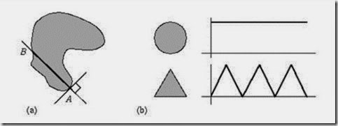
The signature of a region is obtained as a sequence of normal contour distances. The normal contour distance is calculated for each boundary element as a function of the path length. For each border point A, the shortest distance to an opposite border point B is sought in a direction perpendicular to the border tangent at point A (Fig 9). Signatures may be applied to the recognition of overlapping objects or whenever only partial contours are available.
Fig 9: Signature (a) Construction (b) Signatures for a circle and a triangle
o Chord distribution
Chord is a line joining any two points of the region boundary. Distribution of lengths and angles of all chords on a contour may be used for shape description.
Let b(x, y) = 1 represent the contour points, and b(x, y) = 0 represent all other points. The chord distribution can be computed (Fig 10(a)) as


Comments
Post a Comment