Convex hull and Algorithm: Region convex hull construction

Convex hull

• A region R is convex if and only if for any two points x1, x2 from R, the whole line segment defined by its end-points x1, x2is inside the region R.

• The convex hull of a region is the smallest convex region H which satisfies the condition R is a subset of H.

• The convex hull has some special properties in digital data which do not exist in the continuous case. For instance, concave parts can appear and disappear in digital data due to rotation, and therefore the convex hull is not rotation invariant in digital space.

• The convex hull can be used to describe region shape properties and can be used to build a tree structure of region concavity.

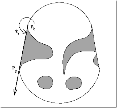
Fig 23: Convex hull

• A discrete convex hull can be defined by the following algorithm which may also be used for convex hull construction.

o This algorithm has complexity O(n2) and is presented here as an intuitive way of detecting the convex hull.

Algorithm: Region convex hull construction

1. Find all pixels of a region R with the minimum row co-ordinate; among them, find the pixel P1 with the minimum column co-ordinate.

Assign Pk = P1, v= (0, 1); the vector v represents the direction of the previous line segment of the convex hull.

2. Search the region boundary in an anti-clockwise direction and compute the angle orientation cpn for every boundary point Pn which lies after the point P1(in the direction of boundary search-see Fig 4). The angle orientation cpn is the angle of vector Pk Pn . The point Pq satisfying the condition cpq = minn cpn is an element (vertex) of the region convex hull.

3. Assign v = PkPq , Pk = Pq .

4. Repeat steps 2 and 3 until Pk = P1 .

• More efficient algorithms exist, especially if the object is defined by an ordered sequence of n vertices representing a polygonal boundary of the object.

• If the polygon P is a simple polygon (self-non-intersecting polygon) which is

always the case in a polygonal representation of object borders, the convex hull may be found in linear time O(n).

• In the past two decades, many linear-time convex hull detection algorithms have been published, however more than half of them were later discovered to be incorrect with counter-examples published.

• The simplest correct convex hull algorithm was developed by Melkman and is now discussed further.

o Let the polygon for which the convex hull is to be determined be a simple polygon P = v1, v2, ⋯ vn and let the vertices be processed in

this order.

o For any three vertices x, y, z in an ordered sequence, a directional function delta may be evaluated

Fig 24: Directional function 8. (a) 8(x, y, z) = 1. (b) 8(x, y, z) = 0. (c) 8(x, y, z) = −1.

• The main data structure H is a list of vertices (deque) of polygonal vertices already processed.

• The current contents of H represents the convex hull of the currently

processed part of the polygon, and after the detection is completed, the

convex hull is stored in this data structure.

• Therefore, H always represents a closed polygonal curve, H = {db ... dt} where db points to the bottom of the list and dtpoints to its top.

• Note that db and dtalways refer to the same vertex simultaneously

representing the first and the last vertex of the closed polygon.

• Main ideas of the algorithm:

o The first three vertices A, B, C from the sequence P forms a triangle (if not collinear) and this triangle represents a convex hull of the first three vertices.

o The next vertex D in the sequence is then tested for being located inside or outside the current convex hull.

o If D is located inside, the current convex hull does not change.

o If D is outside of the current convex hull, it must become a new convex hull vertex and based on the current convex hull shape, either none, one, or several vertices must be removed from the current convex hull.

o This process is repeated for all remaining vertices in the sequence P.

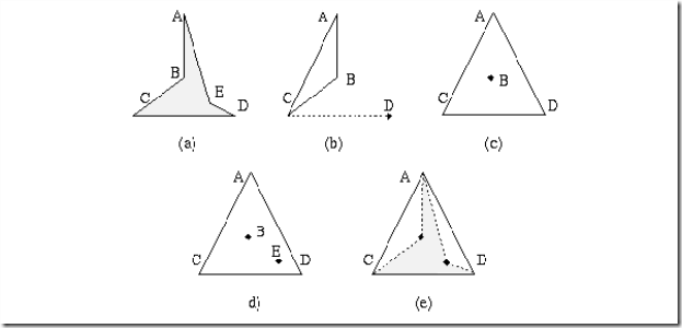
Fig 25: Convex hull detection. (a) First three vertices A, B, C forms a triangle. (b) If the next vertex D is positioned inside the current convex hull ABC, current convex hull does not change. (c) If the next vertex D is outside of the current convex hull, it becomes a new vertex of the new current convex hull ABCDA.

(d) In this case, vertex B must be removed from the current convex hull and the new current hull is ADCA.

• The variable v refers to the input vertex under consideration, and the following operations are defined:

input v ∶ next vertex is entered from sequence P, if P is empty, stop,

• The algorithm is then;

Algorithm: Simple polygon convex hull detection

1. Initialize.

• t ≔ −1;

• b ≔ 0;

• input v1; input v2 ; input v3 ;

• if (o(v1, v2, v3) > 0)

• {pusℎ v1 ;

• pusℎ v2; }

• else

• {pusℎ v2 ;

• pusℎ v1; }

• pusℎ v3 ;

• insert v3;

2. If the next vertex v is inside the current convex hull H , enter and check a new vertex ; otherwise process steps 3 and 4 ;

• input v;

• wℎile (o(v, db , db+1 ) ≥ 0 and o(dt-1, dt , v) ≥ 0)

• input v;

3. Rearrange vertices in, top of the list.

• wℎile(o(dt-1, dt , v) ≤ 0)

• pop dt ;

• pusℎ v ;

4. Rearrange vertices in, bottom of the list.

• wℎile(o(v, db , db+1) = 0)

• remove db

• insert v ;

• go to step 2 ;

• The algorithm as presented may be difficult to follow, however, a less formal version would be impossible to implement.

• The following example makes the algorithm more understandable.

Let P= {A, B, C, D, E} as shown in Fig 7(a). The data structure H is created in the first step;

Based on the values of the directional function o, in this case, no other vertex is entered during this step. Step (3) results in the following current convex hull H;

• A new vertex should be entered from P, however there is no unprocessed vertex in the sequence P and the convex hull generating process stops.

• The resulting convex hull is defined by the sequence

H ={db ,... , dt} = {D, C, A, D} which represents a polygon DCAD, always in the clockwise direction.

Fig 26: Example of convex hull detection. (a) The processed region-polygon ABCDEA. (b) Vertex D is entered and processed. (c) Vertex D becomes a new vertex of the current convex hull ADC. (d) Vertex E is entered and processed E does not become a new vertex of the current convex hull. (e) The resulting convex hull DCAD.

• A region concavity tree is generated recursively during the construction of a convex hull.

• A convex hull of the whole region is constructed first, and convex hulls of concave residua are found next.

• The resulting convex hulls of concave residua of the regions from previous steps are searched until no concave residuum exists.

• The resulting tree is a shape representation of the region.

Fig 27: Concavity tree construction. (a) Convex hull and concave residua. (b) Concavity tree.

Graph representation based on region skeleton

• Objects are represented by a planar graph with nodes representing sub regions resulting from region decomposition, and region shape is then described by the graph properties.

• There are two general approaches to acquiring a graph of sub regions:

o The first one is region thinning leading to the region skeleton, which can be described by a graph.

o The second option starts with the region decomposition into sub regions, which are then represented by nodes while arcs represent neighborhood relations of sub regions.

• Graphical representation of regions has many advantages; the resulting graphs

o are translation and rotation invariant; position and rotation can be

included in the graph definition

o are insensitive to small changes in shape

o are highly invariant with respect to region magnitude

o generate a representation which is understandable

o can easily be used to obtain the information-bearing features of the graph

o are suitable for syntactic recognition

• Graph representation based on region skeleton

• This method corresponds significantly curving points of a region boundary to graph nodes.

• The main disadvantage of boundary-based description methods is that

geometrically close points can be far away from one another when the boundary is described - graphical representation methods overcome this disadvantage.

• The region graph is based on the region skeleton, and the first step is the skeleton construction.

• There are four basic approaches to skeleton construction:

o thinning - iterative removal of region boundary pixels

o wave propagation from the boundary

o detection of local maxima in the distance-transformed image of the region

o analytical methods

• Most thinning procedures repeatedly remove boundary elements until a pixel set with maximum thickness of one or two is found. The following algorithm constructs a skeleton of maximum thickness two.

Algorithm: Skeleton by thinning

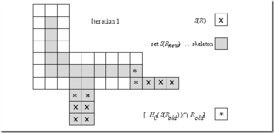
1. Let R be the set of region pixels, Hi (R) its inner boundary, and H0(R) its outer boundary. Let S(R) be a set of pixels from the region R which have all their neighbors in 8-connectivity either from the inner boundary Hi (R) or from the background – from the residuum of R. Assign Rold = R .

2. Construct a region Rnew which is a result of one-step thinning as follows

• Steps of this algorithm are illustrated in the next Figure.

• If there are skeleton segments which have a thickness of two, one extra step can be added to reduce those to a thickness of one, although care must be taken not to break the skeleton connectivity.

Fig 28: Skeleton by thinning

• Thinning is generally a time-consuming process, although sometimes it is not necessary to look for a skeleton, and one side of a parallel boundary can be used for skeleton-like region representation.

• Mathematical morphology is a powerful tool used to find the region skeleton.

• Thinning procedures often use a medial axis transform to construct a region skeleton.

• Under the medial axis definition, the skeleton is the set of all region points which have the same minimum distance from the region boundary for at least two separate boundary points.

• Such a skeleton can be constructed using a distance transform which assigns a value to each region pixel representing its (minimum) distance from the region's boundary.

• The skeleton can be determined as a set of pixels whose distance from the region's border is locally maximal.

• Every skeleton element can be accompanied by information about its distance from the boundary -- this gives the potential to reconstruct a region as an envelope curve of circles with center points at skeleton elements and radii corresponding to the stored distance values.

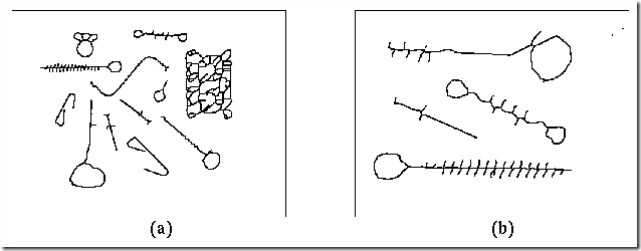
• Small changes in the boundary may cause serious changes in the skeleton.

• This sensitivity can be removed by first representing the region as a polygon, then constructing the skeleton.

• Boundary noise removal can be absorbed into the polygon construction.

• A multi-resolution approach to skeleton construction may also result in decreased sensitivity to boundary noise.

• Similarly, the approach using the Marr-Hildreth edge detector with varying smoothing parameter facilitates scale-based representation of the region's skeleton.

Fig 29: Region skeletons; small change in border can have a significant effect on the skeleton

Fig 30: Region skeletons: Thickened for visibility.

• Skeleton construction algorithms do not result in graphs but the transformation from skeletons to graphs is relatively straightforward.

• Consider first the medial axis skeleton, and assume that a minimum radius

circle has been drawn from each point of the skeleton which has at least one point common with a region boundary.

• Let contact be each contiguous subset of the circle which is common to the

circle and to the boundary.

• If a circle drawn from its center A has one contact only, A is a skeleton end- point.

• If the point A has two contacts, it is a normal skeleton point.

• If A has three or more contacts, the point A is a skeleton node-point.

Algorithm: Region graph construction from skeleton

1. Assign a point description to all skeleton points- end point, node point, and normal point.

2. Let graph node points be all end points and node points. Connect any two graph nodes by a graph edge if they are connected by a sequence of normal points in the region skeleton.

• It can be seen that boundary points of high curvature have the main influence on the graph.

• They are represented by graph nodes, and therefore influence the graph structure.

• If other than medial axis skeletons are used for graph construction, end- points can be defined as skeleton points having just one skeleton neighbor, normal-points as having two skeleton neighbors, and node-points as having at least three skeleton neighbors.

• It is no longer true that node-points are never neighbors and additional

conditions must be used to decide when node-points should be represented as nodes in a graph and when they should not.

Region decomposition

• The decomposition approach is based on the idea that shape recognition is a hierarchical process.

• Shape primitives are defined at the lower level, primitives being the

simplest elements which form the region.

• A graph is constructed at the higher level - nodes result from primitives, arcs describe the mutual primitive relations.

• Convex sets of pixels are one example of simple shape primitives.

Fig 31: Region decomposition (a) Region. (b) Primary regions. (c) Primary sub-regions and kernels. (d) Decomposition graph.

• The solution to the decomposition problem consists of two main steps:

o The first step is to segment a region into simpler sub regions (primitives)

o Second is the analysis of primitives.

• Primitives are simple enough to be successfully described using simple scalar shape properties.

• If sub regions are represented by polygons, graph nodes bear the following information;

1. Node type representing primary sub region or kernel.

2. Number of vertices of the sub region represented by the node.

3. Area of the sub region represented by the node.

4. Main axis direction of the sub region represented by the node.

5. Center of gravity of the sub region represented by the node.

• If a graph is derived using attributes 1-4, the final description is translation invariant.

• A graph derived from attributes 1-3 is translation and rotation invariant.

• Derivation using the first two attributes results in a description which is size invariant in addition to possessing translation and rotation invariance.

Region neighborhood graphs

• Any time region decomposition into sub regions or image decomposition into regions is available, the region or image can be represented by a region neighborhood graph (the region adjacency graph being a special case).

• This graph represents every region as a graph node, and nodes of

neighboring regions are connected by edges.

• A region neighborhood graph can be constructed from a quad tree image representation, from run-length encoded image data, etc.

Fig 32: Binary relation.

• Very often, the relative position of two regions can be used in the description process -- for example, a region A may be positioned to the left of a region B, or above B, or close to B, or a region C may lie between regions A and B, etc.

• We know the meaning of all of the given relations if A, B, C are points, but, with the exception of the relation to be close, they can become ambiguous if A, B, C are regions.

• For instance, human observers are generally satisfied with the definition:

o The center of gravity of A must be positioned to the left of the leftmost point of B and (logical AND) the rightmost pixel of A must be left of the rightmost pixel of B

Shape classes

• Representation of shape classes is considered a challenging problem of shape description.

• The shape classes are expected to represent the generic shapes of the

objects belonging to the class well and emphasize shape differences between classes, while the shape variations allowed within classes should not influence the description.

• There are many ways to deal with such requirements.

• A widely used representation of in-class shape variations is determination of class-specific regions in the feature space.

• The feature space can be defined using a selection of shape features described earlier.

• Another approach to shape class definition is to use a single prototype shape and determine a planar warping transform that if applied to the prototype produces shapes from the particular class.

• The prototype shape may be derived from examples.

• If a set of landmarks can be identified on the regions belonging to specific shape classes, the landmarks can characterize the classes in a simple and powerful way.

• Landmarks are usually selected as easily recognizable border or region

points.

• For planar shapes, a co-ordinate system can be defined that is invariant to similarity transforms of the plane (rotation, translation, scaling).

• If such a landmark model uses n points per 2D object, the dimensionality of the shape space is 2n.

• Clearly, only a subset of the entire shape space corresponds to each shape class and the shape class definition reduces to the definition of the shape space subsets.

• Cootes et al. determine principal components in the shape space from training sets of shapes after the shapes are iteratively aligned.

• The first few principal components characterize the most significant variations in shape.

• Thus, a small number of shape parameters represent the major shape variation characteristics associated with the shape class.

Such a shape class representation is referred to as point distribution models.